
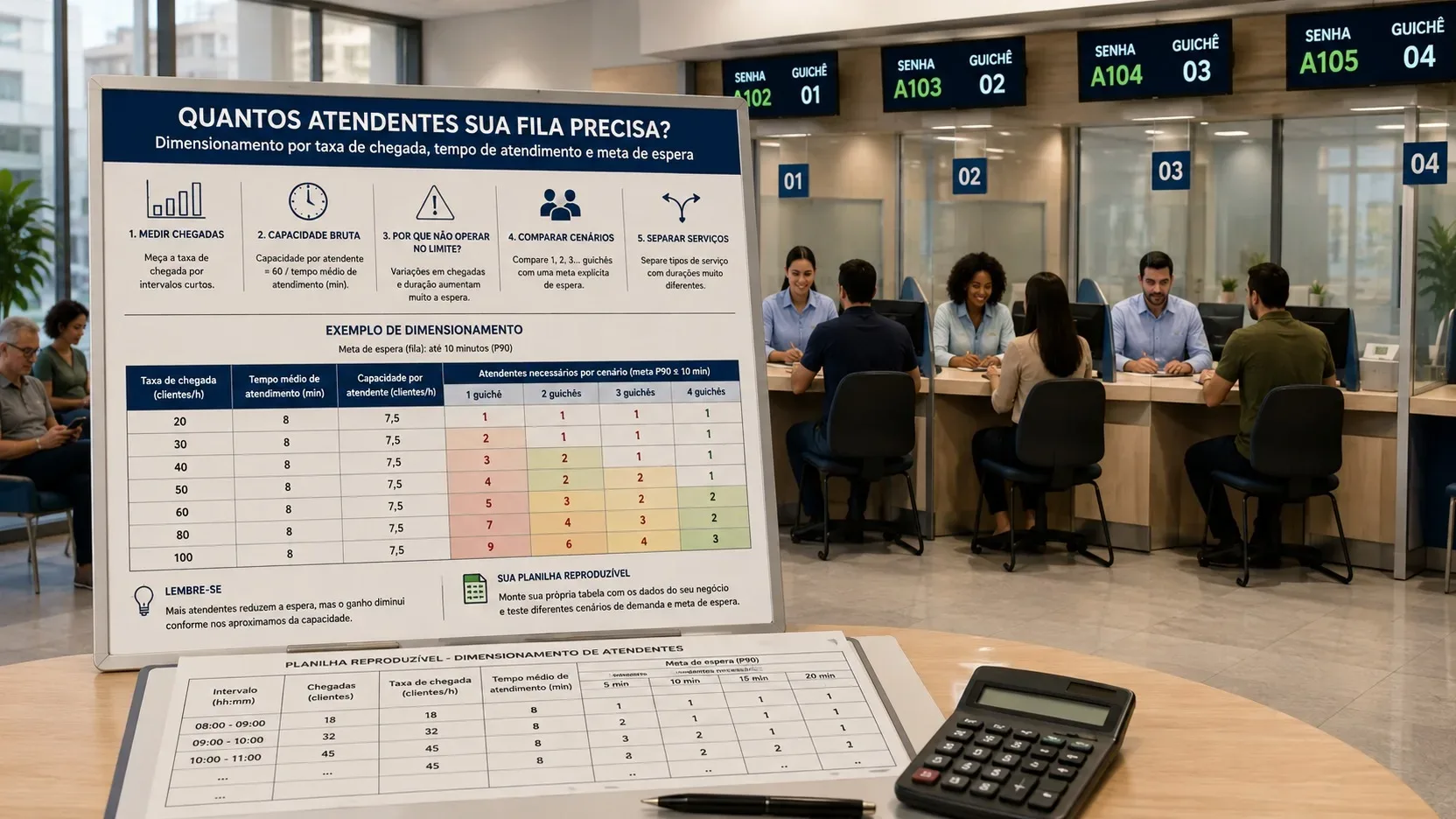
Dividing the volume of customers by the average capacity of an attendant does not alone answer how many counters your queue needs. This account only provides a load reference. When the operation works close to 100% capacity, any variation in arrivals or service duration creates accumulated delay. Useful sizing starts with short intervals, transforms service time into capacity, compares different numbers of attendants and chooses the smallest scenario that meets an explicit waiting target.
Start with the range, not the average for the day
A queue does not feel the daily average; she feels the peak of each period. If 240 people arrive over eight hours, the average of 30 per hour hides the difference between an hour with 15 arrivals and another with 50. To scale, organize the data into intervals that represent the real dynamics of the service, typically 15, 30 or 60 minutes.
At each interval, calculate the equivalent arrival rate per hour. If 15 people arrived in 30 minutes, the rate for that period is 30 arrivals per hour. If 12 arrived in 15 minutes, the equivalent rate is 48 per hour. This conversion allows you to compare demand and capacity in the same unit.
The interval needs to be short enough to reveal peaks, but not so short that any chance turns into a false trend. In operations with very variable flow, 15 or 30 minutes is often a better starting point than an average of several hours. The history must consider comparable days, seasonality, opening times, holidays, campaigns and other events that change arrival.
Transform service time into gross capacity
If the average service time, or TMA, is 8 minutes, the theoretical capacity of an attendant is 60 divided by 8, or 7.5 services per hour. This number is the service fee per attendant, which can be called mu.
The load offered to the queue can be calculated by: load = arrival rate x TMA / 60. With 30 arrivals per hour and a TMA of 8 minutes, the load is 4. This means that, on average, there are four attendant-hours of work required each hour.
This load should not be confused with the final number of attendants. In a simple queue model with waiting and no abandonment, the system is only stable when the number of attendants is greater than the load. In the example, four attendants represent exactly 100% theoretical occupancy. There is no capacity left to absorb the randomness of arrivals and services, so the queue does not have a long-term balance at this point. Five attendants are the first stable scenario, but we still don't know if they meet the waiting target.
Why operating at the limit is fragile
Queues arise because customers do not arrive at perfectly regular intervals and services do not all end at the same time. The greater the occupancy, the less slack there is to absorb this variation. Therefore, waiting time increases non-linearly when utilization approaches 100%.
This effect also makes prediction important. If the scale was set up for 95% occupancy and the actual demand is only 5% above forecast, the effective utilization is very close to 100%. The team may have been correctly sized for the expected average and still produce excessive waiting on a slightly busier day.
The objective, therefore, is not to choose a universal occupancy percentage. It involves defining a service goal and testing how many attendants are needed to reach it with the demand and the TMA of the interval.
Define the waiting target before choosing the number of counters
An operational goal needs to say what an acceptable wait means. Examples are: 90% of customers begin service within 10 minutes; average wait below 5 minutes; or P90 for a wait of up to 10 minutes. These metrics are not equivalent.
For sizing, a target such as percentage met within a period of time is especially practical. Saying that 90% must begin service within 10 minutes is equivalent to demanding that, in the model, the probability of waiting more than 10 minutes is at most 10%.
The choice of the goal is managerial. Urgent care may require much less tolerance than a service in which the customer agrees to wait. Calculation transforms this decision into capacity; it does not alone decide what level of service is appropriate.
Compare scenarios with Erlang C when assumptions are reasonable
The Erlang C model is a classic reference for queues with multiple parallel servers. In basic form, it assumes arrivals according to a Poisson process, independent service times with exponential distribution, equivalent attendants, first-come, first-served service discipline and customers who do not leave the queue before being served.
Within these assumptions, use lambda for the arrival rate per hour, mu for the capacity per attendant per hour, c for the number of attendants and a for the load offered, where a = lambda / mu. The usage is rho = a/c. If rho is greater than or equal to 1, discard the scenario for an unbounded, no-abandon queue because it is not stable.
For each stable c, Erlang C calculates the probability of a customer finding all agents busy and needing to wait. With this probability, it is also possible to calculate the chance that the wait will exceed time t and, therefore, verify a target such as 90% within 10 minutes.
The reproducible form is this. First calculate the denominator as the sum of a to the power of k divided by k factorial, for k from zero to c minus one, plus the term a to the power of c divided by c factorial and by 1 minus rho. Then, the probability of waiting is the second term divided by the denominator. The average wait in line is the probability of waiting divided by (c times mu minus lambda). Finally, the service level up to time t is 1 minus the probability of waiting multiplied by exp of minus (c times mu minus lambda) times t, using t in the same unit of time as the rates.
Example: 30 arrivals per hour and TMA of 8 minutes
With a TMA of 8 minutes, each attendant has an average capacity of 7.5 calls per hour. With 30 arrivals per hour, the load offered is 4.
With four attendants, rho is 1. The scenario operates at the theoretical limit and is not stable in Erlang C. With five attendants, rho drops to 0.80. The calculation gives a waiting probability of approximately 55.4%, an average wait of approximately 4.43 minutes and approximately 84.1% of customers starting service
in up to 10 minutes.
With six attendants, rho drops to approximately 0.667. The probability of waiting is around 28.5%, the average wait drops to around 1.14 minutes and approximately 97.7% of customers begin service within 10 minutes.
If the goal is 90% within 10 minutes, five attendants are not enough in this example, while six attendants meet the goal under the model's assumptions. A simple division of demand by capacity would indicate four, exactly the scenario that has no room for variability. This difference is the reason for not treating gross capacity as final sizing.
Use Little's Law as a check, not as a scaling formula
Little's Law relates three averages: number of customers in the system, arrival rate and average time in the system. In simple form, L = lambda x W. The same relationship can be applied to the queue, using the average number of people waiting and the average waiting time.
It is very useful for checking whether the data makes sense. If the arrival rate is known and the system records an average waiting time, the relationship helps estimate how many people should, on average, be in line. But it does not determine how many attendants are needed to meet a percentile or a waiting target. To do this, you need to model the variability and number of servers.
Separate services with very different durations
A single average can hide mixtures that produce very distinct queues. Imagine that one counter does a 3-minute procedure and another takes 20 minutes. A global TMA may even represent the total load, but it does not show how the distribution of times affects waiting or whether attendants have the same skills to perform both services.
When types of service have very different durations, priorities or competencies, calculate volume and time by type. Then decide whether the queues actually share the same team. If any attendant can treat any customer, there is a gain in capacity sharing. If certain counters are specialized, each group must be sized according to the demand it can actually meet.
It is also important to separate service time from unavailable time. Breaks, shift changes, conferences, administrative tasks, system unavailability and rework reduce effective capacity. The number of open windows is not necessarily equal to the number of productive agents during the entire interval.
When Erlang C should not be used alone
Erlang C is an approximation, not a complete snapshot of the operation. It loses accuracy when the pattern of arrivals changes greatly within the interval itself, when customers abandon the queue, when there are strong priorities, when attendants have different skills, when service times are very asymmetrical, when there are arrivals in batches or when capacity changes during the period.
If abandonment is relevant, models like Erlang A may represent limited patience. If the queue mixes various types of customers and skills, multi-class models or discrete event simulation are often more appropriate. When demand varies rapidly, a simulation of historical arrivals and service times can show effects that a stationary interval account does not capture.
A safe practice is to use Erlang C as a baseline when the assumptions are acceptable and then compare the prediction with the actual operation. If the model says the wait should be low and the observed data remains high, look for broken assumptions before simply adding people.
Build a spreadsheet that can be recalculated at each interval
Each line of the spreadsheet must represent a time interval and contain, at a minimum, the beginning and end of the period, number of arrivals, equivalent arrival rate per hour, TMA, capacity per attendant, load offered and the c scenarios you want to test. For each scenario, calculate rho and discard rho greater than or equal to 1.
In the following columns, calculate the probability of waiting for Erlang C, the average wait and the service level for the defined goal. The decision line is the smallest c that meets the criterion. Repeat the process for all intervals of the day. The result is not a single number of agents for the company, but a curve of need over time.
Then apply a scale layer. Queue sizing tells you how many attendants need to be available at each interval. The scale transforms this need into real shifts, considering breaks, lunch, training, absenteeism, working hours limits and activities that take people away from work. Confusing these two steps is another common source of undersizing.
Work with base, peak and uncertainty scenarios
Don't just use a historical average lambda value. Set up at least one typical scenario and one peak scenario consistent with history. In sensitive operations, add a margin for forecast error or use a demand quantile from the range rather than just the average.
The same logic applies to TMA. If it changes by time, day or type of service, use specific estimates. If a process change has recently reduced the TMA, do not mix old and new months as if they were the same operation.
The value of the spreadsheet is in making the hypotheses explicit. When demand rises, the TMA changes or the waiting target becomes more demanding, the recommended number of attendants changes in front of the manager, without depending on a hidden magic formula.
How to take advantage of data already registered in Biomi Pass
Biomi Pass' public documentation informs that the operation records status, times, counter, type, reason and history of transitions. It also informs that the reports bring together volumes, absences, cancellations and times, and that solutions by sector display waiting and service reports.
This data forms a suitable basis for building the spreadsheet by interval: volume feeds lambda, times feed TMA and separation by type or sector helps not to mix services with different profiles. Before calculating, confirm how the system defines each duration, for example if the time includes transfer, pause, active service or completion, so as not to compare metrics with different meanings.
The final number is a service level decision
The smallest number of attendants capable of processing the load is not necessarily the number that delivers the desired experience. Right sizing has two separate questions. The first is how many attendants are needed for the queue to be stable. The second is how many there are
necessary to meet the waiting target with sufficient margin for actual variability.
Start with data at short intervals, convert AMR to capacity, calculate load, rule out scenarios at the limit, test window numbers against an explicit target, and validate the prediction with observed behavior. This process produces a justifiable and comparable scale over time, rather than a number chosen by the day's average.